
- Prior knowledge
- The hardware
- The goal
- Terminology and symbols
- My requirements for a good renderer
- A quick aside on 3D mathematics
- The general algorithm
- Simplifying the mathematics
- The simplified algorithm
- Optimisations
- Source code
- Speed of the renderer
- Evaluation and next steps
- Acknowledgements
- References
- External links
The Mode 6 pseudo-3D renderer - how was it done?
This article concerns the idea, algorithm and implementation behind the Mode 6 graphics engine used in the ZX Spectrum game, Cosmic Payback.
Prior knowledge
This article strives to explain the concepts necessary to understand the functioning of the renderer; however, some prior knowledge of basic algebra will be required to make sense of the mathematics. Additionally, familiarity with Z80 machine code, though not necessary (unless you decide to inspect the source code), will help somewhat.
The hardware
The Sinclair ZX Spectrum, introduced to the market on the 23rd of April 1982, is fairly underpowered when it comes to graphics. All that it provides is a 1-bit 256x192 framebuffer, with a 32x24 colour attribute overlay [1]. Unlike its main rival, the Commodore 64, there are no hardware sprites, nor a character mode, so the display must be manipulated entirely in software. This wouldn't be a challenge if it weren't for the CPU: a Zilog Z80A operating at 3.5MHz [1]. Though it performs decently for sprite games, 3D graphics of any type are a challenge, given the lack of in-built multiplication and division instructions.
The goal
My original idea was to have a fully textured 3D environment with three degrees of movement (left-right, forward-back and yaw); similar to those found in SNES games such as Super Mario Kart. During the planning stage, I came to realise that this would likely be infeasible, so I removed the rotation ability, leaving two degrees of movement. A slower puzzle/exploration style game would be better suited to such an engine.
I had trouble devising a method of implementing fast perspective-correct texture mapping, so I reduced the plans further to include just filled polygons. This seemed more doable given the restrictions of the machine, but I knew that a traditional approach to 3D rendering would not allow for a satisfactory framerate.
Conventional real-time 3D rendering involves an environment constructed of polygons. The 3D points making up the environment are projected into a 2D space using perspective projection formulae. From these 2D points, the polygons can be drawn to the display. Of course, this is a very simplified explanation, but it is enough to appreciate why achieving 3D graphics on the Spectrum this way is incredibly difficult to achieve at the speeds required for interactivity: there are simply too many calculations required.
Freescape, the engine devised by Alternative Software and used in games such as Driller and Castle Master, gives the player six degrees of freedom – they can look side-to-side, up and down, move the camera viewpoint and even tilt it. However, Freescape suffers from abysmal frame rates. Conversely, games such as I, of the Mask and Micronaut One, written by Sandy White and Pete Cooke respectively, feature fast polygonal 3D graphics, but in both games, this comes at the cost of scene complexity and freedom of movement.
Due to the computational overhead of calculating each vertex and filling polygons according to their bounds, I instead pursued a different method of rendition, which would involve drawing the scene on a per-scanline basis, scanning across the environment tile map and writing pixels accordingly. This finally seemed realistic, but it would still be a considerable challenge.
Terminology and symbols
Before I begin to describe the algorithm, I want to define the terminology and symbols which I will refer to in this article, so as to be as clear as possible:
- Tile map – the two-dimensional grid of square blocks from which the 3D image is derived.
- Viewport – the on-screen window which contains the 3D image.
- Scanline – refers to a single horizontal run of the 3D viewport (note that this does not necessarily correspond exactly to a scanline of the computer's video display).
- Row – a horizontal line of tiles in the tile map.
- Segment – a section of texture which is drawn to a scanline.
- T-state – a single pulse of the Z80 CPU's clock. These are generally used to calculate the time it will take for a set of instructions to execute. Each instruction takes a minimum of 4 T-states to execute [2]. On the ZX Spectrum, each T-state takes 1/3,500,000th of a second [1].
- \( x_{m} ,\ y_{m} ,\ z_{m} \) – the map pointer's X, Y and Z coordinates respectively (\( y_m = -42.5 \) in the implementation used in Cosmic Payback)
- \( x_{p} ,\ z_{p} \) – the player object's X and Z coordinates respectively
- \( x_{c} ,\ y_{c} ,\ z_{c} \) – the camera object's X, Y and Z coordinates respectively (\( x_{c} ,\ z_{c} \) are offset from the player's coordinates by arbitrary amounts, which are unimportant in the consideration of the rendering algorithm, while \( y_{c} = 0 \) )
- \( x_{v} ,\ y_{v} \) – the viewport X and Y coordinates respectively
- \( y_{horizon}\) – the Y position of the horizon within the viewport
- \( w_{v} ,\ w_{s} ,\ w_{s_{c}}\) – the width of the viewport, a segment representing a single tile on the current scanline, and the running total of segment widths respectively
- \( \{x\} \) – notation used to denote the fractional part of \( x \)
My requirements for a good renderer
Obviously, for a playable game, it's no good rendering to a tiny window at a laughably poor frame rate. There has to be a baseline of quality for an acceptable experience:
- High resolution – Ideally, the rendering elements (the smallest unit that can be manipulated in the 3D viewport) should not be so large as to be distinctly visible (i.e. blocky). The viewport should be as large as is feasibly possible. With our use-case, we can cheat a bit by only rendering the bottom half of the screen, since the scene has a horizon in the middle.
- Fast – for a smooth experience, the game should run at an average of 17 frames per second (approx. 60ms per frame). Rendering should therefore take at most 2 video frames worth of CPU time (approx. 40ms, or 140,000 T-states). This will allow for a frame of copying the viewport buffer to the screen and processing game logic.
- Detailed – there should be facilities to allow for the definition of individual tiles using a pattern fill, either static or animated.
A quick aside on 3D mathematics
 Our investigation of the renderer involves as little mathematics as possible. The derivation of the width of a segment, and consequently the X position of our map pointer, can be reverse-engineered from a concept image. Indeed, that is how I wrote the algorithm to compute those variables. It is more difficult, however, to determine empirically how to calculate the Y position of the map pointer, so we will instead use perspective projection formulae and adapt them to our needs.
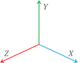
Suppose we have a camera at the origin of our 3D coordinate system (i.e. \( X_{c} =Y_{c} =Z_{c} =0 \)), and we want to project a point at \( (X,Y,Z) \) to a position on the screen \( (X',Y') \). Assuming the distance from the camera to the screen is one unit, the formulae to determine the position on the screen are:
$$ X'=\frac{X}{Z} ,\ Y'=\frac{Y}{Z} $$
We want to work backwards from a Y coordinate on the screen to a point in 3D space. If we rearrange the latter equation, we get:
$$ Z=\frac{Y}{Y'} $$
Ordinarily, we would be left with Y as an unknown, meaning we would be unable to work backwards from an arbitrary point on the screen to a point in 3D space. However, since our tile map plane is the only object in the space, and we know its Y coordinate, we can substitute this into the equation to give us our Z coordinate.
Of course, these formulae use a screen space where the centre of the screen is the origin. To fix our Z equation, we need to subtract the number of scanlines to the horizon, because our viewpoint coordinate system has the origin in the bottom-left (so X increases as you go right, and Y increases as you go up):
$$ Z=\frac{Y}{Y'-Y'_{horizon}} $$
If you would like to take a deeper dive into the formulae underpinning this type of 3D rendering, then I recommend that you read J. Vijn's "Mode 7" tutorial, linked in reference [3].
The general algorithm
Before we begin to pick apart the renderer to speed it up, it is best that we understand what it is essentially doing by examining an unoptimised version of the algorithm. Though our final algorithm will be entirely different in its method of computation, it will be functionally equivalent. Note that this article is not concerned with the technicalities of copying the finished image to the screen, nor overlaying sprites onto the viewport – that is a different, albeit shorter, subject altogether.
In short, our renderer works by processing each scanline of the viewport in sequence, first calculating the starting position within the tile map for that scanline (taking into account the 3D perspective we wish to achieve), and then scanning over the tile map to determine what line segments to draw, until the end of the current scanline is reached.
- For \( y_{v} \) = 0 to 39,
- Compute the new segment width: \( w_{s} =w_{s_{min}} +\frac{y_{v}}{y_{v_{max}}} \cdot ( w_{s_{max}} -w_{s_{min}}) \)
- Calculate the X coordinate of the map pointer using the formula: \( x_{m} =x_{c} -\frac{w_{v}}{2w_{s}} \)
- Calculate the Z coordinate of the map pointer using the formula: \( z_{m} =\frac{y_{c}}{y_{v} -y_{horizon}} \)
- Find the width of the first segment using the formula: \( w_{s_{1}} =w_{s} \cdot ( 1-\{x\}) \)
- Until we reach the right-hand edge of the current scanline:
- Draw the segment to the screen at \( (v_{x} ,v_{y}) \) with width \( w_{s_{t}} \)
- \( x_{m} =x_{m} +1 \)
Simplifying the mathematics
In order to reduce the computation required to render a frame, we must find a way to reduce the amount of operations required, either through pre-calculation or outright removal.
- X coordinate calculations – Because we know in advance what the X coordinate of the map pointer will be on each scanline (relative to the camera's coordinates), we can simply pre-calculate the values and store them in a lookup table. In my implementation, the table contains the difference from the previous value, making the per-scanline calculation a simple addition to the current map pointer coordinate; storing them as offsets from the player coordinates works just as well.
- Z coordinate calculations – As with the X coordinates, the Z coordinate of the map pointer is the same for each line every time the renderer is run (relative to the player's coordinates). This calculation could also be replaced with a lookup table, but instead I elected to use a method which involved simple addition. For each scanline of the viewport, we simply add a delta value (call it \( \delta Z_{m} \)) to the Z coordinate of the map pointer, and then increment \( \delta Z_{m} \). This gives the illusion of depth without the table, albeit with the disadvantage of a small but tolerable amount of distortion [4].
- Segment width calculations – The segment widths can be calculated very simply – since the width of the segment decreases by a constant amount for each scanline, we can reduce the calculation to a simple subtraction from a running total.
- Combining identical tiles – By scanning across the map to identify runs of identical tiles, we can combine their individual segments into one longer segment, meaning that we eliminate the computational cost of the setup work for the extra segments. This turned out to be quite a major breakthrough, as the average use case includes many runs of identical tiles.
The simplified algorithm
Below is the outline of our rendering algorithm, after having applied the changes summarised above. Unlike its previous iteration, this version of the algorithm only requires one multiplication per scanline, of which our viewport has 40.
- Calculate initial map scanner coordinates from player coordinates
- For \( y_{v} \) = 0 to 39,
- Subtract the necessary amount from \( x_{m} \), determined by the lookup table
- Compute the new Z coordinate for the map pointer: \( z_{m} =z_{m} +\delta z_{m} ,\ \delta z_{m} =\delta z_{m} +1 \),
- Compute the new tile segment width: \( w_{s} =w_{s} -\delta w_{s} \), where \( \delta w_{s} \) is the difference in segment width per scanline.
- Find the width of the first segment using the formula: \( w_{s_{t}} =w_{s} \cdot ( 1-\{x_{c}\}) \)
- Until we reach the end of the current scanline:
- \( x_{m} =x_{m} +1 \)
- If the tile at the map pointer is identical to that of the current run, then \( w_{s_{t}} =w_{s_{t}} +w_{s} \)
- If the tile at the map pointer is not identical to that of the current run OR the current run has exceeded the width of the screen:
- Draw the segment to the screen at \( (v_{x} ,v_{y}) \) with width \( w_{s_{t}} \)
- \( x_{m} =x_{m} + w_{s_{t}} , w_{s_{t}} = w_{s} \)
Optimisations
Our algorithm has now been stripped to the bare-bones, computation-wise. However, unless our implementation is similarly efficient, then our renderer could still run like treacle. In this section, we will discuss some techniques to allow our code to really run at lightning speed, relatively speaking. Be aware that this section is about algorithmic optimisations – the annotated source-code listing reveals the more CPU-specific optimisations (i.e. register allocation, instruction replacement) that were carried out as the last step of speeding up the renderer.
Number format
Since our renderer does not require a great deal of precision, we can get away with using fixed-point mathematics for the sections that need non-integer values. An 8.8 format (where the whole and fractional parts of a number are assigned 8 bits each) will fit comfortably into the 16-bit register pairs of the Z80, and also allows for the simple separation of the whole and fractional parts, since each part occupies a byte exactly.
Multiplication
A fairly standard multiplication routine, taking 2 8-bit operands and returning a 16-bit result, will require at most 415 T-states [5]. Even with the multiplications minimised in quantity, this is still too slow; 415*40 = 16600 T-states, which is around 12% of the absolute maximum T-state budget. We could reduce this figure significantly by implementing quarter-square multiplication. This particular method of multiplication uses an identity of the special products [6]:
$$ \left\lfloor \frac{( x+y)^{2}}{4}\right\rfloor -\left\lfloor \frac{( x-y)^{2}}{4}\right\rfloor =\frac{1}{4}\left(\left( x^{2} +2xy+y^{2}\right) -\left( x^{2} -2xy+y^{2}\right)\right) =\frac{1}{4}( 4xy) =xy $$
This method requires 512 bytes for the quarter-square lookup table, but in return, we achieve a significant speed-up, with the new routine only taking 124 T-states to execute in all cases. In order for the routine to work, however, it must be guaranteed that \( ( x+y) \) and \( ( x-y) \) are both within the range of a signed 8-bit integer, that being between -128 and 127. Hence, the operands are truncated to ensure this is the case, with the result being scaled back up after the multiplication. In practice, only the player's X coordinate is truncated, since the whole part of the segment width is small enough to be unproblematic. Truncation comes at the cost of losing some accuracy – the end result is effectively 14-bit. This can manifest itself as tiles having "ragged" edges (i.e. edges that are not exactly straight).
Memory organisation
We can achieve speed gains if we restructure our memory layout so as to reduce the calculations necessary to compute the addresses of required data.
- Texture pattern structure – We can arrange our texture pattern data so that we only need to increment the high-byte of the address to get to the next line of texture, an operation that is faster to perform than adding an arbitrary number to the address.
- Buffer reorganisation – Since the renderer works from left-to-right on each scanline, we can reorganize the viewport buffer so that the address of the next scanline follows on from the end of the previous scanline. This means we will only have to ever increment our viewport pointer, saving us T-states and meaning we don't have to reserve any CPU registers for an addition operation. This will mean that our image is effectively rendered "upside-down", but we can flip it the right way up when we copy the buffer to display memory.
Segment drawing routine
A segment is a run of texture, bounded by two edges on the left and right. Due to the nature of the Spectrum's display layout, where each bit controls a single pixel, we must perform "masking" when the edge of a segment does not correspond exactly to a byte boundary. See the below figure for a graphical representation of this organisation and the masking operation.
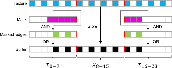
So, we can split the majority of segments into three sections: the left edge, the central run of texture, and the right edge. We can speed up the rendering of segments in several ways:
- Inlining – Instead of calling out to a separate segment drawing routine and putting up with the concomitant overhead, we can instead include the code within the main body of the renderer. This doesn't require any extra memory, since the routine only gets called from one area in the code.
- Maintaining reused values – Instead of recalculating values that will be the same from one segment to the next, we can instead organize our register usage to allow us to keep them. In the case of the Mode 6 renderer, the pointer to the current display byte within the viewport buffer is the same between consecutive segments, since the renderer works sequentially across a scanline. The mask for the start of a new segment will be the inverse of the mask for the edge of the last segment's end – this simple trick of inverting the previous mask allows us to halve the total amount of mask calculations.
- Unrolled loops – Rather than wasting time and registers keeping track of how many bytes we have left to fill, we can repeat the "fill byte" sequence for as many bytes as there are in a scanline. Then, we simply make a jump so that we start mid-way through the loop and only copy as many bytes as necessary.
- Mask table – Mask bytes can be pre-calculated and stored in a table for quick access. This requires only 8 bytes for the lookup table, but saves a great deal of processing time, since we do not have to laboriously loop and set bits in the right places.
Source code
For the sake of brevity, this listing includes only the code for the main rendering loop, leaving out the setup code and definitions for variables, equates and lookup tables. You can visit the GitHub repository to obtain the full source code.
ld hl,m6_gfxbuffer-1 exx m6_render_newline: ; We have reached a new line, so let's set up the registers for the next loop ld a,(m6_render_row) inc a ; Increment loop counter cp 41 ; All rows rendered? ret nc ; ...then exit the renderer ld (m6_render_row),a ld l,a ; Make copy of row number ld a,(m6_render_dy) ; Get delta Y inc a ; Increment delta Y ld (m6_render_dy),a ; Store new delta Y in memory m6_render_newline_l1: ; Keep delta Y in the shadow accumulator for now ex af,af' ld a,l exx ; LINE SET ================================= push hl ; Save buffer address ; Now calculate graphics page ld l,a and 3 add a,m6_tiledata/256 ld ixh,a ; Calculate page for this line of graphics ; Add offset for the delta table ld a,l add a,0+(m6_centretab-1)%256 ld l,a adc a,0+(m6_centretab-1)/256 sub l ld h,a ; Form address to centre table ld e,(hl) ; Get delta from memory ld d,0 ; Extend to 16-bit (could've optimised by ; using 8 to 16 trick a few lines above) ld hl,(m6_render_x) ld a,h ; For later comparison add hl,de ; Add delta ld (m6_render_x),hl cp h ; Change? call nz,m6_render_map_left ; Adjust map pointer if so ; Now let's process our Y coord using our delta Y from the shadow accumulator ex af,af' ld hl,(m6_render_y) add a,l ld l,a call c,m6_render_map_up ; Adjust map pointer on overflow to MSB ld (m6_render_y),a ; Store LSB ; Prepare the line set pop hl ; Restore buffer address inc hl ; Move up a line ld (hl),d ; Zero out left-hand column ld de,$02ff exx ; MAP SET ================================== ; Now retrieve width ld hl,(m6_render_width) ld de,m6_render_dw add hl,de ex de,hl ld (m6_render_width),de ; Multiply the high byte of the width by the fractional component of X using the quarter-square ; multiplication technique. This routine has been adapted from an article in issue 92 of the ; "MSX Computer and Club Webmagazine" push de ; Make a copy of width ld a,(m6_render_x) ; Load LSB of camera position srl a srl a ; Truncate to 6 bits ld e,a ; Get inverted fractional part sub d ; Work out (a-b) ld h,m6_multab/256 ld l,a ; Form address to quarter-square table ld c,(hl) inc h ld b,(hl) ; Load ((a-b)^2)/4 into BC ld a,e add a,d ; Work out (a+b) ld l,a ld e,(hl) dec h ld l,(hl) ld h,e ; Load ((a+b)^2)/4 into HL ; N.B. Ordinarily, OR A would be required before the SBC instructionto prevent a carry flag mishap. ; However, the carry was reset by the ADD A,D instruction a few lines ago sbc hl,bc ; Result = ((a+b)^2)/4 - ((a-b)^2)/4 add hl,hl add hl,hl ; Scale back up to account for truncation ; Now add an extra bit of accuracy pop de ; Restore segment width ld a,(m6_render_x) bit 1,a jr z,m6_render_newline_l2 ld a,l add a,d ld l,a adc a,h sub l ld h,a m6_render_newline_l2: ; Initialise the other registers ld bc,(m6_render_map) ; Get current map address ld a,(bc) ; Get tile dec c ; Move to next tile - first tile guraranteed ; to be a match ld (m6_render_core_comparison_smc+1),a ; Set current run for first tile of row ; Now prepare the map set. We must calculate the partial width m6_render_core: ; This is the core rendering loop. Here, we keep checking map tiles until we hit a different tile. ; Then, we draw the segment representing that run of map tiles. ld a,(bc) ; Get map byte m6_render_core_comparison_smc: cp 0 ; Current byte? (self-modifying code) jr nz,m6_render_core_l2 ; Exit loop if not m6_render_core_l1: ; Bytes match, so add width to right edge. dec c ; Advance map pointer add hl,de ; Add width to segment jp nc,m6_render_core ; Jump back if no overflow ; The edge counter has overflowed, so we must have hit the end of this row. We need ; to draw the last segment, and then we can move up a row. ld h,255 ; Clip right edge to screen boundary m6_render_core_l2: ; Now we must get the pattern byte and draw the segment in question ld a,(m6_render_core_comparison_smc+1) ; Get run m6_render_core_tile_smc: add a,0 ; Add animation index (self-modifying code) ld ixl,a ; Store in IXL ld a,h ; Copy right edge to A exx ; LINE SET ================================= ld c,a and 7 ; Keep bit-wise position ld iyl,a ; Form address to edge table ld a,c rrca rrca rrca and 31 ; Keep byte-wise portion ld b,a inc b ; This will set the carry flag for lines inc b ; with no run of bytes in the middle sub d ; Subtract left edge ld d,b ; Copy new edge to left edge jp c,m6_render_core_edge ; Jump ahead for edge handling ; We have worked out the width of the central run in bytes, so now to adjust the ; upcoming relative jump for the filling code add a,a ; Double run length cpl add a,63 ; Equivalent to subtracting from 64 ld (m6_render_core_jump_smc+1),a ; Store offset ld c,(ix+0) ; Load texture byte ld a,e ; Get old mask and c ; AND against texture byte or (hl) ; OR to the buffer ld (hl),a ; Store back in buffer m6_render_core_jump_smc: ; This part is the filling stage, which copies the raw line graphic into the buffer jr $ ; (self-modifying code) rept 32 inc l ; Next byte of buffer ld (hl),c ; Copy pattern byte into buffer endm inc l m6_render_core_l3: ld a,(iy+0) ; Get new edge mask ld e,a cpl ; Invert mask and c ; AND against graphic ld (hl),a ; Load into buffer m6_render_core_endline: ; We have now plotted our line, so do some clean up work for the next one exx ; MAP SET ================================== ld a,(bc) ; Grab tile ld (m6_render_core_comparison_smc+1),a ; Store new tile into comparison ld a,255 cp h ; End of screen? jp nz,m6_render_core_l1 ; Not overflowed, so loop back jp m6_render_newline ; Now for next line of buffer m6_render_core_edge: ; This branch handles lines made up of only two edges (16 - 9px) inc a ; Just a small edge case? jr nz,m6_render_core_edge_single ; This must be a double edge situation. ld c,(ix+0) ; Load texture byte ld a,e ; Get old mask and c ; AND against texture byte or (hl) ; OR to the buffer ld (hl),a ; Store back in buffer inc l m6_render_core_edge_left: ld a,(iy+0) ; Get new edge mask ld e,a cpl ; Invert mask and c ; AND against graphic ld (hl),a ; Load into buffer jp m6_render_core_endline m6_render_core_edge_single: ; This must be a single edge situation ld a,c ld c,(ix+0) ; Load texture byte inc a ; Check X coordinate of right edge jr nz,m6_render_core_edge_left ; Jump behind if byte is on left side ld a,e ; Get old mask and c ; AND against texture byte or (hl) ; OR to the buffer ld (hl),a ; Store back in buffer jp m6_render_core_endline
Speed of the renderer
 During initial tests, the renderer took on average 4 to 5 video frames of processing time to construct an image. This was during my earlier, more optimistic tests where the renderer was programmed to show 80 scanlines. After I halved the number of scanlines to 40, the mean render time fell to under 2 video frames, or around 90,000 T-states to be more precise. This fell quite comfortably within my T-state budget – even the algorithms worst case scenario, a checkerboard pattern with no consecutive identical tiles, caps out at 130,000 T-states. To maintain the same aspect ratio as before, the 40 scanlines of the viewport are doubled to 80 when they are copied to display memory.
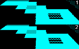
The execution times recorded were better than expected, so I was able to make small adjustments to the multiplication routine that would allow it to calculate the result with an extra binary digit of accuracy, at the cost of a slight slowdown (63 T-states worst case, 55.5 on average). This very slight increase in computation time resulted in a significant reduction of the "ragged edge" effect, improving the visual quality of the rendered images in a small but not insignificant way; compare the straightness of the edges in the two images on the right to appreciate the difference.
Evaluation and next steps
Overall, I am fairly satisfied with my work on the Mode 6 renderer; it is probably the project of which I am proudest so far. If I were to take this renderer further, I might look into adding texture-mapping or rotation – even almost a year after writing this engine, I'm still not sure if either of these would be feasible on the 48K Spectrum at the speeds I would like, though they are no doubt doable on a more powerful clone machine, such as the Spectrum Next, with its native multiply instructions and software overclocking to 28MHz [7]. If anything, it proves to me that filled pseudo-3D graphics can be achieved with some bodging and still look convincing enough to be enjoyable – this may act as my impetus for further experiments.
Acknowledgements
I would like to thank the following people, who have aided me in the production of this article.
- Jonathan Stringer for kindly sacrificing his time to help with proofreading
References
| [1] | M. Korth, "Sinclair ZX Specifications," 2001-2012. [Online]. Available: https://problemkaputt.de/zxdocs.htm. [Accessed 16 May 2021]. |
| [2] | Zilog, Inc., "Z80 CPU User Manual," August 2016. [Online]. Available: http://www.zilog.com/docs/z80/um0080.pdf. [Accessed 21 May 2021]. |
| [3] | J. Vijn, "Tonc: Mode 7 Part 1," 8 April 2010. [Online]. Available: https://www.coranac.com/tonc/text/mode7.htm. [Accessed 14 May 2021]. |
| [4] | L. Gorenfeld, "Lou's Pseudo 3d Page," 2013. [Online]. Available: http://www.extentofthejam.com/pseudo/. [Accessed 15 May 2021]. |
| [5] | z80 Heaven, "Math," [Online]. Available: http://z80-heaven.wikidot.com/math. [Accessed 10 May 2021]. |
| [6] | MSX Computer & Club Webmagazine, "Multiplication on a Z80," 2000. [Online]. Available: https://www.msxcomputermagazine.nl/mccw/92/Multiplication/en.html. [Accessed 14 May 2021]. |
| [7] | ZX Spectrum Next Official Developer Wiki, "Specifications," [Online]. Available: https://wiki.specnext.dev/Specifications. [Accessed 11 May 2021]. |
External links
- The GitHub repository containing the full source code for the Mode 6 renderer